Data Browser
Overview
The Data Browser is a trending tool. It can display the values of ‘live’ Process Variables (PVs) as well as historic data in a Stripchart-type plot over time.
- Live Data
For each PV, the Data Browser collects ‘live’ samples from the control system and plots them over time. The size of the live sample buffer is configurable, as is the sample period.
- Historic Data
The Data Browser queries archive data sources for historic samples to obtain data for time ranges ‘before’ the live sample buffer. You can configure one or more archive data source for each PV.
Getting Started
To create a new plot:
Invoke the menu
Applications,Display,
Data Browser.Open the plot’s context menu by right-clicking into the plot, invoke

Add PV.Enter the desired PV name, press “OK”.
Plot Configuration .plt Files
Use the File, Save menu entry or the keyboard shortcut
CTRL + S (CMD + S on Mac OS) to save the plot settings, which include
PV names, trace colors and axis arrangements.
The default file extension for plot files is .plt.
You can later re-open the configuration by opening the .plt file,
adjust settings, for example axis ranges, and save the updated configuration.
The .plt files store the configuration of a plot, but no data.
To save an image of the current plot, use Save Snapshot from the plot context menu item.
To save the data shown in the plot, refer to the “Exporting Data” section below.
Note that any zooming or panning of a plot changes the plot settings,
so when then closing the plot, you will be prompted to save the updated settings.
This may not be desirable in an operational setup. For example, assume a .plt file was
created with a time axis range that displays the last 6 hours. When users
open this configuration, they are free to zoom in or out, even add or remove traces,
but when they close the plot, you may not want them to overwrite the original settings.
There are two ways to accomplish this.
One is the “Save Changes” option in the plot’s “Properties Panel” described below.
The other is making the .plt file read-only using operating system file tools
or the CS-Studio File Browser. Configuration files can also be loaded via HTTP links,
which are always read-only. When trying to close a plot with modified configuration,
the Data Browser noticed if the original file cannot be written and will prompt
with a “Save-As” dialog to offer saving to a new file.
Toolbar
Open the plot’s tool bar by right-clicking into the plot,
then invoke ![]()
Show Toolbar.
Stagger
The ![]()
Stagger button will set the range of each value axis
such that the traces on different axes don’t overlap.
In other words, all the traces of the first value axis will appear on top,
followed by the traces on the second axis below,
the traces on the third axis below the second axis and so on.
Zooming
The buttons to ![]()
Zoom In and ![]()
Zoom Out
activate the respective zoom mode.
While in Zoom In mode,
pressing the mouse on a start point in the time axis, then dragging to an end point in the time axis and finally releasing the mouse button will zoom into the selected time region.
similarly selecting a start..end range on a value axis will zoom into the selected range on that value axis.
dragging a rectangle inside the plot will zoom into the selected region
While in Zoom Out mode,
clicking the mouse on the time axis zooms out of that point in time.
clicking the mouse on a value axis zooms out of that value on that axis.
clicking the mouse inside the plot zooms out of that point on the time axis and all value axes.
Zoom In can also be activated within the plot by simply holding
the Control key, then dragging a range on the time axis,
value axis or within the plot.
Finally, while the mouse pointer is within an axis or the plot,
you can hold the Control key and then use the scroll wheel
to zoom in or out of an axis or the plot.
Properties Panel
Open the plot’s property panel by right-clicking into the plot,
then invoke ![]()
Open Properties Panel.
The panel allows you to configure each trace, the time axis, the value axes, and miscellaneous settings. Changes performed in this panel will be persisted when the plot (.plt) file is saved.
The meaning of most options should become evident by simply using them, with a few exceptions.
On the “Misc.” tab, “Plot redraw period” and “Scroll Step” control how the plot updates and scrolls. For example, a redraw period of 1 and a scroll step of 10 refreshes the plot every second, while scrolling the time axis every 10 seconds. This makes for a plot that mostly stands still, only moving every 10 seconds. Larger redraw periods can be useful to reduce CPU usage.
The “Save Changes” option on the “Misc.” tab controls how the plot behaves when closed.
By default, the option is checked, and trying to close a modified plot will open a “Save before closing?” prompt.
In an operational scenario, certain plots may be provided with default settings that are not meant
to be overwritten. For those, un-check the “Save Changes” option. Users can now open the plot,
zoom, pan, even add or remove traces, and then simply close the plot without a prompt, preserving
the desired default settings. Note that when you un-check the “Save Changes” option to get this
behavior, you already activated it, so you need to use “Save As” from the File menu to save
the *.plt file with the un-checked “Save Changes” option.
Context Menu
One or more traces in the trace tab of the property panel can be selected using Shift + click or Control (Windows)/ Command (Mac) + click.
By right click, the context menu opens.
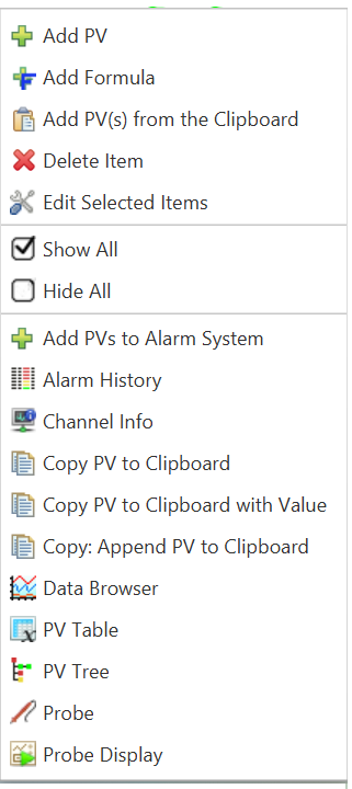
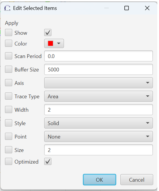
Among other funcionality, multiple selected items can be edited in a dialog by clicking Edit Selected Items.
Runtime Properties Dialog
If enabled through the preference setting org.csstudio.trends.databrowser3/config_dialog_supported, plot settings may
also be changed using the runtime properties dialog. To launch the dialog, click on the plot area and then press letter “o”:
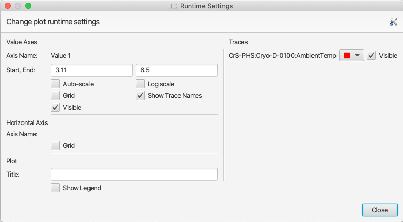
NOTE: changes to the plot performed from the runtime properties dialog will not update the data model constructed from the underlying plot file. Consequently such changes are not persisted when the plot file is saved. To make sure plot properties are saved one must perform the changes in the property panel.
Live Data Sampling
By default, traces will use a Scan Period of 0 seconds, which means
we keep every sample received from the control system.
To avoid running out of memory, the live data buffer has a limited
Buffer Size.
For example, if your channel updates every 1 second, and the buffer size
is set to 5000, the data browser will keep roughly the last 1 hour and 20 minutes
of live data in memory. Older samples are dropped.
To keep a longer time span of live data in memory, you can increase the Buffer Size,
which obviously results in using more memory. Alternatively, you can set the Scan Period
to for example 5 seconds. This will ignore the update rate of the channel and simply take
a sample every 5 seconds, allowing a buffer of 5000 samples to hold almost 7 hours of data.
Optimized vs. Raw Archive Data Request
By default, a trace will request Optimized data from an archive.
How this is accomplished depends on the implementation of the underlying
archive system. The fundamental idea is that the data browser
requests a reduced (optimized) set of min/max/average samples.
The number of optimized samples is based on the width of the screen in pixels.
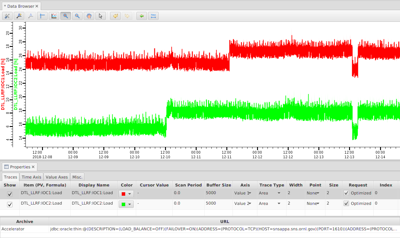
When using ‘Area’ traces as shown below, the average values are
plotted as a line, and the min/max outline is displayed as a
light-colored area. This not only reduces the amount of data compared
to plotting every single raw sample from the archive. In addition it
makes it obvious if a value was fairly stable over time, or if there
was a lot of movement in the data around the average.
Some archive data sources may also provide the standard deviation,
which will be represented as a pair of thinner lines,
one above and one below the thicker average line.
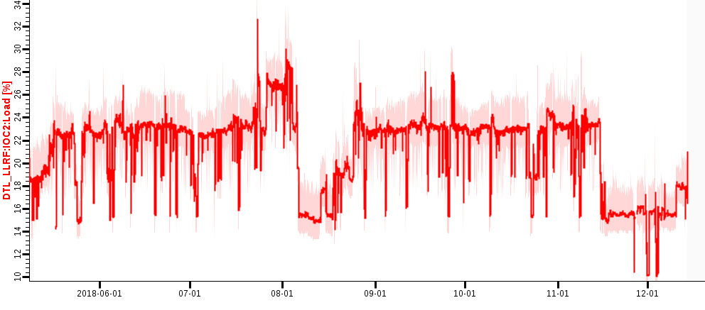
When there are fewer ‘raw’ data points than requested, the ‘Optimized’ algorithm falls back to returning the raw data, meaning: When you zoom into the data far enough, you will eventually get raw data.
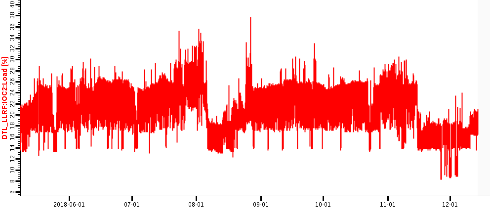
You may use the Request option ofproperty a trace in the property panel
to always request Raw data.
As a result, each original sample is fetched from the archive.
The screenshot below shows the result.
Not only is this usually a larger amount of samples, taking longer to receive and then
to plot. It also uses more memory, and when you try to look at raw
data for a long time range your computer will eventually ran out of
memory. The ‘Raw Data’ requests should therefore only be used when
necessary because of shortcomings in the ‘Optimized’ algorithm.
Trace Types
Ideally, control system data is only updated when it changes by a significant amount. EPICS records actually offer separate update thresholds for live and archived data, so that live displays can receive updates for small changes at the noise level of a signal, while historic data is only written for changes well above the noise level.
When the Data Browser receives either live of historic samples, we assume that those represent significant changes in the value.
The “Area” and “Single Line” Trace Types, shown to the left in the following image, use a stair-step type of line that holds the value of the last sample until a new sample arrives. This reflects our assumption that the signal has not significantly changed until we receive a new sample.


The alternate “Area (direct)” and “Single Line (direct)” Trace Types, shown to the right, draw a direct line between samples, suggesting a linear change of the process variable between known samples.
Exporting Data
Use the “Export” panel to write data into files suitable
for spreadsheet programs or Matlab.
Open the export panel by right-clicking into the plot,
then invoke ![]()
Open Data Export Panel.
- Time Range
By default, the export will use the time range from the plot, but you can export data for a different time range.
- Source Options
By default, the export will fetch raw data from the archive, not the optimized, reduced min/max/average data that is displayed in the plot.
You can modify the time range of the export to differ from the range of the plot, and also select to export either the exact data that is displayed in the plot, or request optimized data with a different number of “bins” from the archive.
Plot: The exact samples currently displayed in the plot will be exported.Raw Archived Data: The exported data will contain data that is requested from the archive without modifications.Optimized Archived Data: To reduce the number of exported samples, optimized data is requested from the archive. You specify the number of desired samples, and the export will then request roughly this number of averaged samples from the archive data source. For example, when requesting 800 optimized samples, the start..end time range is split into 800 “bins”. The the minimum, maximum and average value of the raw samples within each bin is then exported.Linear Interpolation: As an alternative way to reduce the number of exported samples, the exported samples are computed via linear interpolation from the raw data. You specify the interpolation interval in hours, minutes and seconds, for example 00:10:00 to obtain one sample every 10 minutes.- Format Options
The format of the exported file defaults to a spreadsheet suitable for import into most spreadsheet programs. You can modify these settings:
Tabular: Instead of a table that lists the samples for all channels, you can export the samples for each channel separately... with error columns: The min…max range of optimized data is by default exported as “error” columns, suitable for an error-bar display... with Severity/Status: The Severity and Status of each sample is by default exported, but you can omit it if not needed.Default format: The number of decimal digits will be obtained from the data source.Decimal format: You specify the number of decimal digits.Exponential notation: Use exponential notation, where you again specify the number of decimal digits.
Excel Spreadsheets
The exported data files are in a text format with TAB-delimited columns suitable for import into spreadsheet programs like Microsoft Excel.
Assume you chose a filename of “test.dat” on your Desktop, follow these steps for import into Excel:
In Excel, use File/Open to open the file “test.dat”. You might have to select
Files of type: All Files (*.*)in the file “Open” dialog to do this.A “Text Import Wizard” should appear, and the default settings should already be set to
“Delimited - Characters such as … tabs …”
“Delimiters: Tab”
Even though the time stamp column contains the full date and time, Excel will only display time down to minutes, omitting the seconds or microseconds. Fix this by clicking on the “A” table header, i.e. selecting the whole first column; right-click to get the “Format Cells…” dialog, and enter a “Custom” format:
yyyy/m/d h:mm:ss.000
For plots, the “X/Y scatter” plot type using time as the X axis and the value column for the Y axis tends to work best.
Note that Excel is limited to about 65000 lines. If your data file includes more lines, those will be lost in the import. You can work around this by exporting a smaller time range into separate files, or by exporting averaged data.
The value columns for averaged data will contain text like “5 [0… 10]” to indicate that the average value for that time was 5, with a minimum/maximum range of 0 to 10. To perform computations in excel, it might be useful to select the column and perform a text replacement of “[*]” with “” (nothing) to delete the min/max info.
When performing computations on the data, values marked “#N/A” which have non numerical value because they represent a status or error should be ignored by Excel.
OpenOffice.org/LibreOffice Calc Spreadsheets
As long as the exported data file has a “.csv” suffix, OpenOffice.org/LibreOffice should open the file with an “import” dialog similar to MS Excel, where you select “tab” delimited columns as explained above.
File names ending in “.dat”, “.txt” etc. might only open in the OpenOffice.org/LibreOffice Writer (word processor), so you have to use the correct file suffix.
Matlab
The Matlab export can use two different file formats.
To create binary Matlab data files, use a file name ending in .mat.
Matlab text files are created when the file name ends in .m.
The binary data file like “example.mat” is suitable for loading into Matlab 5 and newer like this:
load /path/to/the/example.mat
In your Matlab workspace you should then find structures named “channel0”, “channel1”, …, one for each channel that was loaded from the file. Each structure has the following elements:
name: Channel name
time: Time stamps
value: Numeric value
severity: Severity
The time stamps are saved as text by default. In reasonable modern versions of Matlab you best convert them to Matlab serial date numbers, which you can then for example plot over time like this:
channel0.date = datenum(channel0.time, 'yyyy-mm-dd HH:MM:SS.FFF');
plot(channel0.date, channel0.value);
datetick('x',0);
title(channel0.name);
If user ticks ‘Use UNIX timestamp…’ in the export tab, timestamps will be exported as UNIX timestamp in ms, i.e. as a 64 bit unsigned integer.
The Matlab text files like “example.m” are suitable for loading (executing) in Matlab R2006b or newer, creating one ‘timeseries’ object per trace. To load it into Matlab, you execute the file like this:
cd /path/to/the/file
example
Matlab will then execute the commands in the file which define
the data in the Matlab workspace and also plot it. With Matlab
releases older than R2006b you will have to edit the generated file to
suit your needs, for example use simply plot(v) to show the values.
Command Line Export Options
The export functionality can also be invoked from the command line, without using the graphical user interface. This can be convenient when regularly exporting data for several channels.
To see available options, run phoebus like this:
phoebus -main org.phoebus.archive.Export -help

Usage: -main org.phoebus.archive.Export [options]

Export archived data into files

General command-line options:

-help                                    -  This text
-settings settings.xml                   -  Import settings from file, either exported XML or property file format

Archive Information options:
-list [pattern]                          -  List channel names, with optional pattern ('.', '*')

Data Export options:
-start '2019-01-02 08:00:00'             -  Start time
-end '2019-02-03 16:15:20'               -  End time (defaults to 'now')
-bin bin_count                           -  Export 'optimized' data for given bin count
-linear HH:MM:SS                         -  Export linearly extrapolated data for time intervals
-decimal precision                       -  Decimal format with given precision
-exponential precision                   -  Exponential format with given precision
-nostate                                 -  Do not include status/severity in tab-separated file
-unixTimeStamp                           -  Use UNIX timestamp (in ms) instead of formatted date/time string
-export /path/to/file channel <channels> -  Export data for one or more channels into file

File names ending in *.m or *.mat generate Matlab files.
All other file name endings create tab-separated data files.
The Statistics-tab
Under the Statistics-tab, some basic statistical measures of the plotted data-points can be viewed.
It is important to note that the statistics are calculated only on the data values themselves without taking into account the timestamps of data-points: in the calculation of the statistical measures, only the value of data-points and the total number of data-points are taken into account, while neither the time interval under consideration (except indirectly for determining the subset of data-points to calculate the statistical measures for), nor the timestamps of individual data-points are part of the calculation.
For instance, in a plot based on both archived and live samples, the mean value will be skewed towards the live data portion if live data is sampled at a higher frequency than archived data.